StudySmarter Excel Course: Day 1 = Excel Formulas

Day One: Excel Formulas and Where to Find Them

Does the very thought of Microsoft Excel give you a headache? You’re not the only one. Just like MS Word, Excel can be a moody piece of software, but it’s an exceedingly useful tool for organising just about any amount of information. In our two-day course on Excel formulas and functions, we’ll try to find you a remedy for Excel ailments with a quick and easy overview of the most important features.

PS If the title of our crash course is anything to go by, Excel can be a whole suitcase full of unpredictable beasts that makes you want to smash your head against the keyboard in despair. Luckily enough, we know how to deal with that.

PPS All formulas in Excel start with an equation sign (=) followed by relevant cells and details. 

COUNT Formula in Excel

Name: COUNT

Use frequency: 5/5

Danger: 1/5

COUNT is a simple formula in Excel – it literally counts the number of cells in a selected range. It doesn’t include blank cells or ones with other data besides numbers.

To count in Excel, select the cell where you want the result. In the address bar, type the following:

=COUNT(X1:X35) – Press Enter and you’re done!

X stands for the cell range (the upper horizontal range marked with letters), and the numbers refer to the cell numbers from where you want to start counting to where you want to stop.

To count all information, including textual data, type =COUNTA(X1:X35). To include blank cells, type =COUNTBLANK(X1:X35).

SUM (Addition) and SUBTRACTION Excel Formulas

Name: SUM/SUBTRACTION

Use frequency: 3.5/5

Danger: 1/5

You can do simple addition of two or more cells by writing =A1+A3+A4 or using the SUM formula.

The SUM formula in Excel performs simple addition and calculates the total of the selected range of cells. Skip manual mathematics and pick a cell where you want the result. Then feed the address bar with the following:

=SUM(C1:C4) – Press Enter.

The function will calculate the sum total of the given range.

You can also add selectively with the following formula =SUM(C1+C4+C5) or calculate the sum total of a number of ranges with =SUM(C1-C5,D4:D16). Separate ranges by adding commas between them.

If you want to subtract any numbers, use =A5-A3-A16, etc.

There is no SUBTRACT function in Excel, so if you want a range, you will have to use SUM and add a minus (-) in front of the selected cells you want to subtract, i.e. =SUM(C15,-C12,-C4).

Excel Multiply Formula

Name: Multiplication

Real name: PRODUCT

Use frequency: 3/5

Danger: 3/5 for being crafty

Just like subtraction doesn’t have its own formula and piggybacks on the SUM, multiplication and division borrow from others. You can either do the good old =A5*A6, which can get quite dreary, especially if you have a lot of cells to consider, or you can try the following:

=PRODUCT(A1:A5) which will multiply the said range.

For more complex multiplication, you can add several ranges separated by a comma: =PRODUCT(A1:A5,C2:C4,F14:F16,B2,G1)

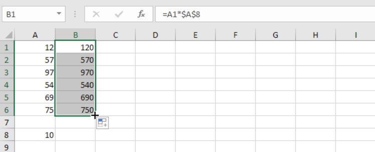
You can also multiply by a constant number by writing that number in a separate cell (best to add a blank somewhere, too, so you don’t forget) and adding the $ sign in front of it:

Here, the constant number is in A8, which is why we have $A$8.

You can also drag the formula down by selecting the first result cell and holding the left click until you’ve selected the range where you want the numbers multiplied by the constant number:

Division Formula in Excel

Division works similarly to multiplication. You add / in the formula, e.g. =A4/A5. You can also select a constant number by adding $ in front of the cell reference.

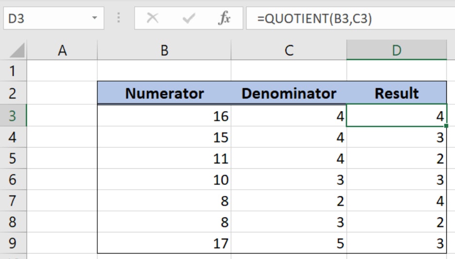
If you don’t want your division to end up with a string of decimal numbers, you can write =QUOTIENT(B4,B3) to return the integer portion of a division or MOD(B4,B3) to return the remainder of the division. Notice the comma rather than slash in this case.

Source

Excel Formulas That Just Do It Better

Let’s face it, addition and subtraction are pretty easy to understand, but unless maths is a part of your daily life, you’ve probably said goodbye to more complex mathematical calculations (I know I have). While you cannot always count on your calculator to help you out – especially if you’re dealing with endless Excel sheets –there are a few more formulas that can make your life easier.

The AVERAGE Formula in Excel

Name: AVERAGE

Use Frequency: Variable

Danger: 4/5, possible shapeshifter

Sometimes you need to find the average number of the selected range (as an administration-hating lecturer, I can promise you I hate calculating average grades, but Excel does help).

The basic idea is simple: =AVERAGE(C4:C15)

AVERAGE automatically excludes blank cells, but sometimes you might find it under the name AVERAGEIF, which looks kinda like this: =AVERAGEIF(B3:D3,”>0″), which will also exclude zeroes because the 0 specifies that you’re looking for values higher than zero.

You can calculate averages manually by typing =SUM(range)/COUNT(range).

Percentage Formula in Excel

I was never much of a fan of calculating percentages, especially in chemistry classes. Thankfully, I don’t have to do it anymore. Still, there may come a time you have to force your MS Excel to do it for you.

Name: Percentage

Use Frequency: 2/5

Danger: 4/5

You can calculate the percentage using the regular formula (part/whole)*100. In Excel, that looks like this:

=A2/A1

When you get the result, multiply it by 100 and you’ll get the percentage.

Alternatively, you can calculate the =A2/A1 and click CTRL+SHIFT+% or % on the Home tab to get the percentage of the calculated amount.

IF Formula in Excel

Name: IF

Use frequency 4/5

Danger: 55555555555555555555555555/5

There are some formulas that should be banned, right?

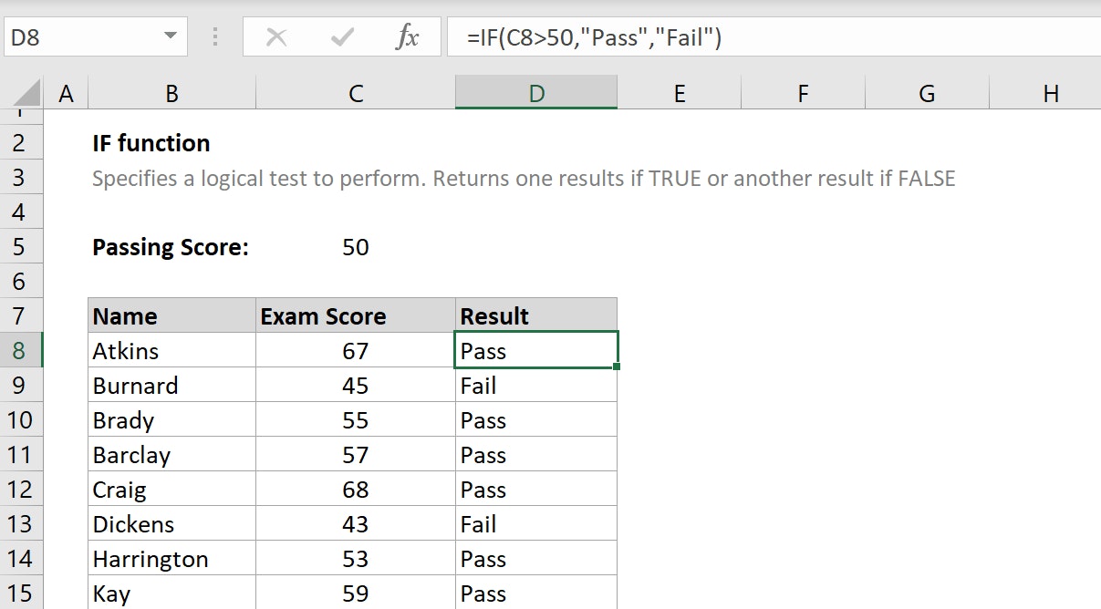
IF is used to specify conditions under which something is calculated, accepted, dismissed, or processed in any other way. There are two results of your IF statement: the first is TRUE if the conditions are met, and the second is FALSE.

=IF(C2=”Yes”,1,2)

This means that if C2 says YES, the formula returns to 1, and if not, it returns to 2.

=IF(C9=”Apple”,TRUE,FALSE)

You can combine IF with other formulas and functions:

=IF(A2>C4,Passed,Failed).

This means that if the value A2 (say a student’s points on the test) is higher than C4 (minimum points for a pass), the text will say Passed in the selected column. Otherwise, it will be marked as failed. Life is cruel sometimes.

How Excel Formulas Scrambled My Brain

And with that, my young Padawan, we complete the first day of the two-day Excel crash course. Remember, Excel formulas are used to calculate anything and everything. They are always marked by = at the beginning, and, if you’ve written them correctly, give you the result when you press enter.

Remember, Excel tends to ignore blank spaces, so you need to specify if you need them included in the calculations.

In our next round of scrambling our brains with higher mathematics, we’ll deal with functions. In the meantime, take a break – you probably need one. I know I do 😉.